SELFE Home
SELFE v3.1d User Manual
- Mandatory input files (needed for all runs):
- Horizontal grid (hgrid.gr3)
- Vertical grid (vgrid.in)
- Boundary condition and tidal info (bctides.in)
- Parameter input (param.in)
- Interpolation mode:
interpol.gr3
- Optional input files (driven by param.in):
- Initial condition for salinity and
temperature (salt.ic,
temp.ic, and ts.ic)
- Bottom drag (drag.gr3
or rough.gr3)
- wind (wind.th)
- Time history
input (flux.th etc.)
- Space- and
time-varying time history inputs (*3D.th)
- adv.gr3
-
Kriging flags (krvel.gr3)
-
Min. and max. diffusivity (diffmin.gr3 and diffmax.gr3)
- Surface mixing length (xlsc.gr3)
- Lat/long
coordinates (hgrid.ll)
- Heat exchange (sflux/)
- Conservation
check files (fluxflag.gr3)
- vvd.dat,
hvd.mom, and hvd.tran
- Amplitudes
and phases of boundary forcings
- Nodal
factor and equilibrium arguments
- Hot
start input (hotstart.in)
- Bed deformation input (bdef.gr3)
- Station locations for station outputs (station.in)
- Harmonic analysis input (harm.in)
- Nudging inputs ([t,s]_nudge.gr3, [temp,salt]_nu.in)
- Output files:
- Run
info output (mirror.out)
- Global output
- Warning
and fatal messages
Input files
Horizontal grid
(hgrid.gr3):
In xmgredit grid format.
Here is an example; below are explanations of format with this grid:
|
hgrid.gr3 ! alphanumeric description
60356 31082 !
of elements and nodes in the horizontal grid
!Following is coordinate
part:
1 402672.000000 282928.000000 2.0000000e+01
! node #, x,y, depth
2 402416.000000 283385.000000 2.0000000e+01
3 402289.443000 282708.750000 2.0000000e+01
4 402014.597000 283185.897000 2.0000000e+01
.............................................
31082 331118.598253 112401.547031 2.3000000e-01 !last node
! Following is connectivity
part:
1 3 1 2 3 ! element #,
element type (triangles only), node 1, node 2, node 3
2 3 2 4 3
3 3 4 5 3
...........................................
60356 3 26914 30943 26804 !last element
|
 |
!Following is boundary condition
part (needed for hgrid.gr3 only):
3 : Number of open boundaries
95 ! Total number of open boundary nodes
3 ! Number of nodes for open boundary 1
29835 ! first node on this segment
29834 ! 2nd node on this segment
29836 ! 3rd node on this segment
90 !Number of nodes for open boundary 2
........................................
2 ! last node on this open segment
16 ! number of land boundaries
1743 ! Total number of land boundary nodes (including islands)
753 0 ! Number of nodes for land boundary 1 ('0' means the exterior boundary)
30381 ! first node on this segment
30380
.......................................
1 !last node on this segment
741 0 ! Number of nodes for land boundary 2 ('0' means the exterior boundary)
.......................................
10 1 ! Number of nodes for island boundary 1 ('1' means island)
29448 ! first node on this island
29451
29525
.......................................
29449 !last node on this island (which is different from the first node above)
.......................................
Note: (1) the boundary condition (b.c.) part can be generated with xmgredit5 --> GridDEM
--> Create open/land boundaries; it can also be generated with SMS;
(2) if you have no open boundary, you can create two land boundary segments
that are linked to each other. Likewise, if you have no land boundary,
you should create two open boundary segments that are connected to each other;
(3) although not required, we recommend you follow the following convention when genrating the
boundary segments. For the exterior boundary (open+land), go in counter-clockwise direction;
for interior boundaries (islands), go in clockwise direction;
(3) The use of a
Shapiro filter (indvel=0 or -1) places some constraints on the boundary sides. In particular, the
center of any internal sides must be inside the quad formed by the centers of
its 4 adjacent sides (see Fig. 1). If not, the code will try to enlarge the
stencil, but if the side is near the boundary, fatal error will occur. To find
out all violating boundary elements, just prepare hgrid.gr3 (note that the open
boundary info needs no be correct at this stage), vgrid.in and param.in up to
ihorcon, and run the code with ipre=1 in param.in. You'll find a list of all
such sides in fort.11 (the two node numbers of a side will be shown). Method to
eliminate this problem includes: (1) move node, (2) swap the side for a pair of
elements, and (3) refine or coarsen. Note that in most grid editors, the first 2
methods won't change the node numbering and so you'd try them first before
Method (3), to save time. After the pre-processing run is successful (with a
screen message indicating so), you can then proceed to prepare other inputs.
If you use xmgredit5 (inside the ACE package), it can help you identify the elements/sides
that need editing. Under the manual:
Edit--> Edit over grid/regions --> Mark Shapiro filter violations,
turn it on and you'll see some elements are highlighted. Not all those
elements need to be edited - only those "pointing" outside the boundary.

go back
Vertical grid (vgrid.in)
This version uses hybrid S-Z coordinates in the vertical, with S on top of Z.
54 18 100. !nvrt; kz (# of Z-levels); h_s (transition depth between S and Z)
Z levels !Z-levels first
1 -5000. !level index, z-coordinates
2 -2300.
3 -1800.
4 -1400.
5 -1000.
6 -770.
7 -570.
8 -470.
9 -390.
10 -340.
11 -290.
12 -240.
13 -190.
14 -140.
15 -120.
16 -110.
17 -105.
18 -100. !z-coordinate of the last Z-level must be -h_s
S levels !S-levels below
30. 0.7 10. ! constants used in S-coordinates: h_c, theta_b, theta_f (see notes
below)
18 -1. !first S-level (S-coordinate must be -1)
19 -0.972222 !levels index, S-coordinate
20 -0.944444
.......
54 0. !last
S-coordinate must be 0
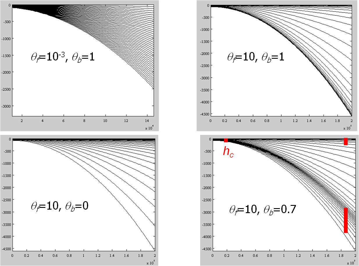
Notes:
- Origin of the vertical axis is at MSL;
- h_c, theta_b, theta_f: constants used in Song and Haidvogel's (1994)
S-coordinate system. h_c
controls surface/bottom boundary layer thickness that requires fine resolution;
theta_f-->0 leads to traditional sigma-coordinates, while theta_f >> 1
skews resolution towards surface and/or bottom; theta_b=1 leads to both
bottom and surface being resolved, while theta_b=0 resolves only surface (see the plot above).
- Global output is from the bottom (variable in space) to surface (level nvrt)
at each node;
- If a "pure S" model is desired, use only 1 Z-level and set h_s to a very
large number (e.g., 1.e6).
- Distribution of z levels at various depths can be seen from the output sample_z.out.
go back
Boundary conditions and tidal info (bctides.in)
Please refer to sample files of bctides.in included in the source code bundle while you read the following.
-
48-character
start time info string, e.g., 04/23/2002 00:00:00 PST (only used for
visualization with xmvis)
-
ntip, tip_dp: # of constituents used in earth tidal potential;
cut-off depth for applying
tidal
potential (i.e., it is not calculated when depth <
tip_dp).
-
For k=1, ntip
talpha(k) = tidal
constituent name;
jspc(k), tamp(k), tfreq(k),
tnf(k), tear(k) = tidal species # (0: declinational; 1: diurnal; 2:
semi-diurnal), amplitude constants, frequency,
nodal factor, earth equilibrium argument (in degrees);
end for;
-
nbfr
= total # of tidal boundary forcing frequencies.
-
For
k=1, nbfr
alpha(k)
= tidal constituent name;
amig(k), ff(k), face(k) = forcing frequency,
nodal factor, earth equilibrium argument (in degrees) for constituents
forced on the open boundary;
end
for;
-
nope: # of open boundary segments;
-
For
j=1, nope
neta(j),
iettype(j), ifltype(j), itetype(j), isatype(j) = # of nodes on the open
boundary segment j (from hgrid.gr3), b.c. flags for elevation, normal velocity, temperature,
and salinity;
if (iettype(j) == 1) !time history of
elevation on this boundary
no input in this file; time history of elevation is read in from
elev.th;
else if (iettype(j)
== 2) !this boundary is forced by a constant elevation
ethconst: constant
elevation
else if (iettype(j)
== 3) !this boundary is forced by tides
for k=1, nbfr
alpha(k) = tidal constituent name;
for i=1,
neta(j)
emo(ieta(j,i),k), efa(ieta(j,i),k) !amplitude and phase for
each node on this open boundary;
end for
end for;
else
if (iettype(j) == 4) !space- and
time-varying input
no input in this file; time history of elevation is read in from
elev3D.th;
else
if (iettype(j) == 0)
elevations are not specified for this boundary (in this case the velocity
must be specified).
endif
if (ifltype(j)
== 0) !nornal vel. not specified
no input needed
else if (ifltype(j) == 1) !time history of
discharge on this boundary
no input in this file; time history of
discharge
is read
in from flux.th;
else if (ifltype(j)
== 2) !this boundary is forced by a constant discharge
vthconst:
constant discharge (note that a negative number means inflow)
else if (ifltype(j)
== 3) !vel. is forced in frequency domain
for k=1, nbfr
vmo(j,k),vfa(j,k) !uniform amplitude and phase along each boundary segment
end for;
else if (ifltype(j)
== 4 or -4) !3D input
no input in this
file; time history of velocity is read
in from uv3D.th.
If ifltype(j)=-4, next line specifies relaxation constants
for inflow and outflow (between 0 and 1 with 1 being strongest nudging).
else if (ifltype(j) == -1) !Flanther type radiation b.c. (iettype must
be 0 in this case)
eta_m0,qthcon(j): mean elevation and discharge on the jth boundary
endif
if (itetype(j)
== 0) !temperature not specified
no input needed
else if (itetype(j) == 1) !time history of
temperature on this boundary
tobc: nudging factor (between 0 and 1 with 1 being strongest nudging) for inflow;
(time history of temperature will be read
in from temp.th;
)
else if (itetype(j)
== 2) !this boundary is forced by a constant temperature
tthconst =
constant temperature
tobc: nudging factor (between 0 and 1) for inflow;
else if (itetype(j)
== 3) !initial temperature profile for inflow
tobc: nudging factor (between 0 and 1) for inflow;
else if(itetype(j)
== 4) !3D input
tobc: nudging factor (between 0 and 1) (time history of
temperature is read in from
temp3D.th);
endif
Salintiy
b.c. is similar to temperature:
if
(isatype(j)
== 0) !salinity not specified
.........
endif
end for !j
- if ntracers /=0, you also need the following for tracer transport.
- itr_met !=1: upwind; 2: TVD
- if(itr_met=2) tvd_mid2,flimiter2 !similar to tvd_met and flimiter for the TVD scheme for transport
nope: # of open boundary segments;
for k=1,nope
- itrtype(k): b.c. type flag
- if(itrtype(k)==2) then !constant values for inflow
trth(1:ntracers,k): imposed values for each tracer
trobc(k): nudging factor between (0,1]
- else if(itrtype(k)==3) then !nudge to i.c. for inflow
trobc(k): nudging factor
- else if(itrtype(k)==0) then !no b.c.
no inputs needed
- endif
end for !k
inu_tr: nudging flag for tracers
if(inu_tr/=0) then
need an input tracer_nudge.gr3 which is similar to t_nudge.gr3;
endif !inu_tr/=0
go back
Parameter input (param.in):
This file uses free format, i.e. the order of each input parameter is not important.
Governing rules for this file are:
- Lines beginning with "!" are comments; blank lines are ignored;
- one line for each parameter in the format: keywords= value;
keywords are case sensitive; spaces allowed between keywords and "=" and value;
comments starting with "!" allowed after value;
- value is an integer, double, or 2-char string (no single quotes needed for string input); for double, any of the format is acceptable:
40 or 40. or 4.e1.
Use of decimal point for integers is OK but discouraged.
Each parameter (and its keyword) is explained as follows; note that you do not have to follow this order.
In some cases we have grouped some parameters for easier explanation, but you should
specify them on separate lines. Refer to sample param.in in the source code bundle.
-
ipre:
pre-processing flag. ipre=1:
code will output centers.bp, sidecenters.bp, obe.out (centers build point,
sidcenters build point, and list of open boundary elements), and
mirror.out and stop. This
is useful also for checking geometry violation, z-levels at various depths (in mirror.out) for any given
choice of vgrid. IMPORTANT: ipre=1 only works for single CPU! ipre=0:
normal run.
-
nonhydro
: Non-hydrostatic model switch (0: hydrostatic model; 1: non-hydrostatic model)
-
im2d: 2D (1) or 3D (0) model.
Note that for 2D model, choice of many parameters will be limited (see the sample param.in);
If im2d=1, theta2 (between [0,1]) specifies the implicitness factor for Coriolis;
-
if nonhydro=1,
ihydro_region: a flag to optionally specify hydrostatic regions in hydro_region.gr3 if ihydro_region=1; 0: all regions are non-hydrostatic;
-
ntracers
: total number of passive tracers.
-
imm: tsunami
option. Default: 0 (no bed deformation); 1: with bed deformation (needs
bdef.gr3); 2: 3D bottom deformation (need to interact with code).
-
If USE_WWM pre-processor is enabled, two parameters are needed to
specify the coupling between SELFE and WWM spectral wave model:
icou_elfe_wwm - 0: no feedback from WWM to SELFE (decoupled);
1: coupled SELFE-WWM; 2: 1-way feedback (radiation stress from WWM to SELFE).
nstep_wwm: call WWM every this many steps in SELFE;
-
imm: tsunami
option. Default: 0 (no bed deformation); 1: with bed deformation (needs
bdef.gr3); 2: 3D bottom deformation (need to interact with code).
-
If imm=1, this
line is ibdef: total # of deformation steps (i.e., the bed will
change from the initial position to the position specified in bdef.gr3 in
ibdef steps).
-
ihot
= hot start flag. If ihot=0, cold start; if ihot/=0, hot start from
hotstart.in. If ihot=1, the time and time step are reset to
zero, and outputs start from t=0 accordingly. If ihot=2, the run (and output) will continue from the time specified in
hotstart.in.
-
ics
= coordinate frame flag. If ics=1, Cartesian coordinates are
used; if ics=2, both hgrid.ll and hgrid.gr3 use degrees latitude/longitude
(and they should be identical to each other).
-
cpp_lon,
cpp_lat= centers of projection used to convert lat/long to Cartesian
coordinates. These are used for ics=2, or a variable Coriolis parameter
is employed (ncor=1), or the heat exchange sub-model is invoked (ihconsv=1).
-
ihorcon: flag to
use non-zero horizontal viscosity. If
ihorcon=0, it
is not used (recommended). If ihorcon/=0, input hvis.gr3 is needed.
-
ihdif: flag to
use non-zero horizontal duffusivity. If
ihdif=0, it
is not used (recommended). If ihdif/=0, input hdif.gr3 is needed.
-
thetai
= implicitness parameter (between 0.5 and 1). Recommended value: 0.6.
-
ibcc,
itransport= barotropic/baroclinic flags. If ibcc=0, a baroclinic model is used
and regardless of the value for itransport, the transport equation is solved. If
ibcc=1, a barotropic model is used, and the transport equation may (when
itransport=1) or may not (when itransport=0) be solved; in the former case, S and T are
treated as passive tracers.
-
If
ibcc=0, the ramp-up fucntion is specified as:
nrampbc,
drampbc: ramp option flag and ramp-up period (in days). If nrampbc=0,
drampbc is not used. A hyperbolic tangent function is used for ramp-up.
-
rnday
= total run time in days.
-
nramp,
dramp = ramp option for the tides and some boundary conditions, and ramp-up
period in days (not used if nramp=0).
-
dt
= time step (in sec).
-
nadv = advection on/off switch. If nadv=0, advection is selectively turned
off based on the input file adv.gr3. If nadv=1 or 2, advection is on for the whole
domain, and backtracking is done using either
Euler
or
5th-order Runge-Kutta (more expensive)
scheme.
-
dtb_max1, dtb_max2: sub-steps used in btrack. For nadv /= 0, only dtb_max1 is used,
which is the minimum sub-step used in Euler scheme (nadv=1) or maximum
sub-step used in
5th-order Runge-Kutta scheme (nadv=2).
For nadv=0, dtb_max1 is the
minimum sub-step used in Euler scheme (when local depth=1 in
adv.gr3) and
dtb_max2 is the
maximum
sub-step used in
5th-order Runge-Kutta scheme
(when
local depth=2 in adv.gr3).
-
h0
= minimum depth (in m) for wetting and drying (recommended value: 1cm). When the total depth is less than h0, the
corresponding nodes/sides/elements are considered dry. It should always be
positive to prevent underflow.
-
bfric
= bottom friction option. If bfric=0, spatially varying drag coefficients are
read in from drag.gr3 (as depth info). For bfric=1, bottom roughnesses (in
meters) are read in from rough.gr3.
-
If
bfric=1, maximum drag coefficient is specified as Cdmax (to prevent
exaggeration of drag coefficient in shallow areas).
-
ncor
= Coriolis option. If ncor=0 or -1, a constant Coriolis parameter is used
(see next line). If ncor=1,
a variable Coriolis parameter, based on a beta-plane approximation, is used,
with the lat/long. coordinates read in from
hgrid.ll.
In this case, the center of CPP projection must be correctly specified (see
above).
-
If
ncor=0, 'coriolis' = constant Coriolis parameter.
If
ncor=-1, 'lattitude' is the mean latitude.
-
nws,
wtiminc = wind forcing options and the interval (in seconds) with which the
wind input is read in. If nws=0, no wind is applied (and wtiminc becomes
immaterial). If nws=1, constant wind is applied to the whole domain at any
given time, and the time history of wind is input from
wind.th. If
nws=2 or 3,
spatially and temporally variable wind is applied and the input consists of a number of
netcdf
files in the directory sflux/. The
option nws=3 is only for checking heat conservation and needs sflux.th.
-
If
nws>0, the ramp-up option is specified as: nrampwind, drampwind = ramp option and period
(in days) for wind.
In addition, the user can scale the wind by using 'iwindoff'. If
iwindoff=0, wind is applied as is. If
iwindoff=1, the scaling factors are the depths in windfactor.gr3.
-
ihconsv,
isconsv = heat budget and salt conservation models flags. If ihconsv=0, the heat budget model is not used. If
ihconsv=1, a heat budget model is invoked, and a number of
netcdf files for radiation flux
input are read in from he directory sflux/.
If
isconsv=1, the evaporation and precipitation model is
evoked but the user needs to turn on the
pre-processing flag PREC_EVAP in Makefile and recompile.
-
itur
= turbulence closure model selection. If itur=0, constant diffusivities are
used for momentum and transport (and the values are specified in the next
line). If itur=-2, vertically homogeneous but horizontally varying
diffusivities are used, which are read in from
hvd.mom.and
hvd.tran. If
itur=-1, horizontally
homogeneous but vertically varying diffusivities are used, which are read in
from vvd.dat.
If itur=2, the
zero-equation Pacanowski and Philander closure is used. If itur=3, then the
two-equation closure schemes (Mellor-Yamada-Galperin, K-epsilon, Umlauf and
Burchard etc.) are used. If itur=4, GOTM
turbulence model is invoked .
-
If
itur=0, the constant viscosity and diffusivity are: dfv0, dfh0.
If itur=2, the next line is: h1_pp, vdmax_pp1, vdmin_pp1,
tdmin_pp1, h2_pp,
vdmax_pp2, vdmin_pp2,tdmin_pp2.
Eddy viscosity is computed as: vdiff=vdiff_max/(1+rich)^2+vdiff_min, and
diffusivity tdiff=vdiff_max/(1+rich)^2+tdiff_min, where rich is a
Richardson number. The limits (vdiff_max, vdiff_min and tdiff_min) vary linearly with
depth between depths h1_pp and h2_pp.
If
itur=3, the next line is:
turb_met, turb_stab:
choice of model description ("MY"-Mellor & Yamada, "KL"-GLS
as k-kl, "KE"-GLS as k-epsilon, "KW"-GLS as k-omega, or "UB"-Umlauf
& Burchard's optimal), and stability function ("GA"-Galperin's,
or "KC"-Kantha & Clayson's for GLS models). In this case, the
minimum and maximum viscosity/diffusivity are specified in
diffmin.gr3 and diffmax.gr3, and the scale for surface mixing
length is specified in xlfs.gr3.
If itur=4, GOTM turbulence model is invoked; the user needs
to compile the GOTM libraries first (see FAQ or README inside GOTM/ for
instructions), and turn on
pre-processing flag USE_GOTM in Makefile and recompile.
The minimum and maximum viscosity/diffusivity are still specified in
diffmin.gr3 and diffmax.gr3,
but xlfs.gr3 is
not needed. In addition, GOTM also requires an input
called gotmturb.inp. There are some ready-made samples for this input in the
source code bundle. If you wish to tune some parameters inside, you may
consult gotm.net for more details.
-
ic_elev: elevation
initial condition flag for cold start. If ic_elev=1, elev.ic (in *.gr3 format) is needed
to specify the initial elevations. Otherwise elevation is initialized to 0 everywhere
(cold start only).
-
icst = options for specifying initial temperature and salinity field
for cold start. If icst=1, a vertically homogeneous but horizontally
varying initial temperature and salinity field is contained in
temp.ic and
salt.ic. If
icst=2, a horizontally
homogeneous but vertically varying initial temperature and salinity
field, prescribed in a series of z-levels, is contained in
ts.ic.
For general 3D initial S,T fields, use the hot start option.
-
ibcc_mean: mean T,S profile option. If ibcc_mean=1 (or ihot=0 and icst=2), mean profile
is read in from ts.ic, and will be removed when calculating baroclinic force.
No ts.ic is needed if ibcc_mean=0.
-
iwrite: output format option; not active and
probably will be removed eventually.
-
nspool,
ihfskip: Global output skips. Output is done every nspool steps, and
a new output stack is opened every ihfskip steps.
Therefore the outputs are named as [1,2,3,...]_[process id]_salt.63 etc.
-
next
25+ lines are global output (in machine-dependent binary) options. The (process-specific)
outputs share similar
structure. Only the first line is detailed here.
-
elev.61 = global
elevation output
control. If
'elev.61' =0, no global elevation is recorded. If 'elev.61'=
1, global elevation for each
node in the grid is recorded in [1,2,3...]_[process id]_elev.61 in binary format.
The
output is either starting from scratch or appended to existing ones
depending on ihot.
-
pres.61: output options for atmospheric pressure (*pres.61).
-
airt.61: output
options for air temperature (*airt.61).
-
shum.61: output
options for specific humidity (*shum.61).
-
srad.61: output
options for solar radiation (*srad.61).
-
flsu.61: output
options for short wave radiation (*flsu.61).
-
fllu.61: output
options for long wave radiation (*fllu.61).
-
radu.61: output
options for upward heat flux (*radu.61).
-
radd.61: output
options for downward flux (*radd.61).
-
flux.61: output
options for total flux (*flux.61).
-
evap.61: output
options for evaporation rate (*evap.61).
-
prcp.61:
output options for precipitation rate (*prcp.61).
-
wind.62: output
options for wind speed (*wind.62).
-
wist.62: output
options for wind stresses (*wist.62).
-
dahv.62: output
options for depth-averaged velocity (*dahv.62).
-
vert.63: output
options for vertical velocity (*vert.63).
-
temp.63: output
options for temperature (*temp.63).
-
salt.63: output
options for salinity (*salt.63).
-
conc.63: output
options for density (*conc.63).
-
tdff.63: output
options for eddy diffusivity (*tdff.63).
-
vdff.63: output
options for eddy viscosity (*vdff.63).
-
kine.63: output
options for turbulent kinetic energy (*kine.63).
-
mixl.63: output
options for macroscale mixing length (*mixl.63).
-
zcor.63: output
options for z coordinates at each node (*zcor.63).
-
qnon.63: output
options for non-hydrostatic pressure at each node (*qnon.63).
-
hvel.64: output
options for horizontal velocity (*hvel.64).
If you use passive tracers and modified the code (ntracer/=0 etc),
the corresponding flags are needed here; e.g., trcr_[1,2,3...].63
If you use WWM, two more output files from WWM are (more coming soon):
- Hsig.61: significant wave height;
- WavD.62: dominant wave direction;
27. testout: output options for test variable (test.60). The user may choose any
internal variable by modifying the source code
iout_sta: station output flag. If iout_sta/=1, an input station.in
is needed.
iharind: harmonic analysis flag. If iharind/=0, an input harm.in
is needed.
hotout,hotout_write = hot start output control parameters. If hotout=0, no hot
start output is generated. If hotout=1, hot start output is spooled to it_[process id]_hotstart every
hotout_write
time steps, where
it is the
corresponding time iteration number, and hotout must be a multiple of ihfskip above. If a run needs to be hot started from step
it, the user needs to combine all process-specific hotstart outputs into a hotstart.in
using combine_hotstart*.f90.
slvr_output_spool,mxitn,tolerance
= parallel JCG solver control parameters.
Recommended
values: 50 1000 1.e-12.
consv_check = parameter for checking
volume and salt conservation. If
turned on (=1), the conservation will be checked in regions specified by
fluxflag.gr3.
inter_st,
inter_mom: linear (inter_st=1) or quadratic (inter_st=2) interpolation for T, S in backtracking,
and linear (inter_mom=0)
or Kriging (inter_mom=1)
for interpolating the velocity
in backtracking. If inter_st=0,
the option is read in from lqk.gr3 as the depth info. If
inter_mom=-1, the depth in krvel.gr3 (0 or 1) will determine the order of
interpolation (linear or Kriging).
depth_zsigma:
Option for computing baroclinic force near bottom. If the local depth
is less than depth_zsigma, constant extrapolation is used; otherwise
a more conservative approach is used to minimze inconsistency.
inu_st,
step_nu, vnh1,vnf1,vnh2,vnf2: nudging flag for S,T, nudging step,
parameters for vertical nudging. When inu_st=0, no nudging is done. When
inu_st=1, nudge to initial conditions. When inu_st=2, nudge to values
specified in temp_nu.in and salt_nu.in, given at an interval of
step_nu.
For inu_st/=0, the horizontal nudging factors are
given
in t_nudge.gr3 and s_nudge.gr3 (as depths info), and the vertical nudging factors vary
linearly along the depth as: min(vnf2,max(vnf1,vnf)),
where vnf=vnf1+(vnf2-vnf1)*(h-vnh1)/(vnh2-vnh1).
The nudging factor is the sum of the two.
idrag: bottom drag option. idrag=1: linear drag formulation; idrag=2:
quadratic drag
formulation (default).
ihhat: wet/dry option. If ihhat=1, the friction-reduced depth will be kept
non-negative to ensure robustness (at the expense of accuracy); if ihhat=0,
the depth is unrestricted.
iupwind_t: upwind option for T,S. A value of "0"
corresponds to Eulerian-Lagrangian transport option (and the interpolation
method is determined by inter_st above), "1" for the
mass-conservative upwind option, and "2" for the higher-order
mass-conservative
TVD scheme (which may be more expensive especially in shallow region).
If the TVD option is invoked for at least one of the variables, then
the TVD method is further specified as: tvd_mid, flimiter.
tvd_mid='AA';
flimiter indicates the choice of flux limiting functions: MM (Minmod);
OS (Osher); VL (Van Leer) or SB (Superbee).
blend_internal,
blend_bnd: blending factors if
indvel=0 or -1 (see below), i.e., discontinuous velocity + Shapiro filter option.
Use 0. 0.
shapiro: filter strength if
indvel=0 or -1(see below).
Recommended: 0.5.
kr_co: choice of generalized covariance function; 1: linear f(h)=-h; 2: (h^2*log(h); 3: (cubic
h^3); 4: (-h^5). See Le Roux (1997) for
details.
rmaxvel: maximum velocity. This is needed mainly for the air-water exchange
as the model may blow up if the water velocity is above 20m^2/s.
velmin_btrack: minimum velocity before backtracking is invoked. e.g., 1.e-3 (m/s).
btrack_noise: set initial noise for backtracking to avoid underflow problem. Must be
between (0,500], and we recommend 100.
inunfl: choice of inundation algorithm.
inunfl=1 can be used if the horizontal resolution is fine enough,
and this is critical for tsunami simulations. Otherwise use inunfl=0. Note that inunfl=1 option is not available at the moment.
indvel: this is an important flag that determines the method of converting
side velocity to node velocity. If
indvel=0 or -1, the node velocity is allowed to be discontinuous across
elements and a Shapiro filter is used to filter out sub-grid noises. If
indvel=1, an averaging procedure is used instead and the node velocity is
continuous across elements. In general,
indvel=0 (or -1) leads to smaller numerical diffusion and dissipation and better
accuracy. But without a velocity boundary condition, this option
will lead to inferior results. If a velocity b.c. is unavailable,
indvel=1 should be used. Note that the geometry check mentioned above will not be performed if indvel=1 is used.
s1_mxnbt, s2_mxnbt: dimensioning parameters used in inter-subdomain
backtracking.
Start from s[12]_mxnbt=0.5 3, and increase them (gradually) if the array size is not enough.
Accuracy is not affected by the choice of these two parameters.
If ntracers>0,
additional lines are needed that specify the transport method (upwind or TVD)
and horizontal boundary conditions etc. Consult the source code for details.
See FAQ for how to interface your own code to SELFE.
go back
Initial condition for S,T
Depending on the values of icst (see parameter input file):
- If icst = 1, salt.ic and temp.ic take the following build point format:
33 to 0 from outh to TP. !file description
30001 !# of nodes;
1 386380.409604 286208.187634 0.000000 !node #, x, y,
initial salinity (or temperature)
2 386460.352736 285995.038877 0.000000
3 386687.720000 286213.590000 0.000000
4 386460.076848 286367.779818 0.000000
5 386678.380000 286483.440000 0.000000
..............
- If icst = 2, ts.ic takes the following format:
43 !total # of vertical levels;
1 -2000. 4. 34. !level #, z-coordinates, temperature, salinity
2 -1000. 5. 34.
3 -500. 6. 33.
4 -200. 7. 32.
5 -100. 8. 31.
...........
go back
Bottom drag (drag.gr3 or
rough.gr3)
grid !file decription
40000
27918 !# of elements, # of nodes
1 386738.500000 285939.060000 0.004500 !node #, x, y, drag coefficient Cd (for
nchi=0) or roughness (in meters; for nchi=1)
2 386687.720000 286213.590000 0.004500
3 386421.090000 286172.160000 0.004500
4 386471.720000 286376.030000 0.004500
5 386678.380000 286483.440000 0.004500
6 386140.190000 286439.220000 0.004500
7 386387.280000 286557.310000 0.004500
8 386209.840000 286676.470000 0.004500
..........
go back
wind (wind.th)
If nws=1 in param.in, a time history of wind speed must be specified in this
file:
5. 8.660254 ! x and y components of wind speed @ 0*wtiminc
5. 8.660254
5. 8.660254
.......
Note that the speed varies linearly in time, and the time interval (wtiminc) is
specified in param.in.
go back
Time history input:
This includes elev.th, flux.th, temp.th, salt.th, which share same structure. Below is a sample
flux.th:
300. -1613.05005 -6186.60156 !time (in sec), discharge at the 1st boundary
with ifltype=1, discharge at the 2nd boundary with ifltype=1
600. -1611.37854 -6208.62549
900. -1609.39612 -6232.22314
1200. -1607.42651 -6254.24707
1500. -1605.45703 -6276.27148
1800. -1603.48743 -6298.2959
2100. -1601.3772 -6321.89307
2400. -1599.40772 -6343.91748
2700. -1597.43811 -6365.94141
3000. -1595.46863 -6387.96582
3300. -1593.49902 -6409.99023
3600. -1591.38879 -6433.5874
3900. -1589.41931 -6452.94287
4200. -1587.2959 -6472.29834
...........
go back
Space- and
time-varying time history inputs (*3D.th):
These include elev3D.th, uv3D.th, temp3D.th, salt3D.th, which share similar
binary structure. For example, uv3D.th:
for it=1,nt !all time steps
read(12,rec=it)time,((uth(k,i),vth(k,i),k=1,nvrt),i=1,nodes); !all open-boundary nodes that need this type of b.c.; time, uth, vth are single precision real.
end for !it
go back
obe.out
This file is generated with the pre-processing flag in param.in for debugging
purpose only.
3 # of open bnd
Element list:
251 bnd # 1
1 31587
2 31588
3 31589
4 31590
5 31592
6 31595
7 31601
8 31603
9 31605
10 31606
........
4 bnd # 2
1 31583
2 31584
3 31585
4 31586
........
go back
adv.gr3
If nadv=0, the advection on/off flags are the "depths" (0: off;
1: Euler; 2: 5th order Runge-Kutta) in this
grid file, which is otherwise similar to hgrid.gr3.
go back
krvel.gr3
The depth specifies the Kriging option for each node: 0 means no Kriging; 1
means applying Kriging there. The order of the generalized covariance function
is specified
in param.in.
go back
Min. and max. diffusivity
The depth specifies the minimum and maximum diffusivity imposed at each
node. This is needed to further constraint outputs from the GLS model. We
generally recommend a constant value of 1.e-6 m^2/s for minimum diffusivity, and
1.e-2 m^2/s for maximum diffusivity inside estuaries and 10 m^2/s otherwise. The
minimum diffusivity may also be changed locally, e.g., to create a mixing pool
near the end of a river.
go back
Surface mixing length
The depth specifies the surface mixing length used when itur=3. It specifies
the portion of surface layer thickness; e.g., 0.5 mean 1/2 of the layer is
used as surface mixing length.
Recommend value: 0.5.
go back
Interpolation mode
The depth specifies the way the vertical interpolation is done locally, i.e.,
along Z or S plane. If the depth=1, it is done along Z-plane; if the depth=2,
along S-plane. We recommend the value of 2 in "pure S" zone, and 1 in SZ zone.
You may not use "2" in the SZ zone.
go back
Lat/long
coordinates (hgrid.ll)
This file is identical to hgrid.gr3 except the x,y coordinates are replaced by
lattitudes and longitudes.
go back
Heat exchange
This consists of a suite of input for wind and radiation fluxes found in
a sub-directory sflux/. When nws=2, the wind speed and atmospheric pressure
are read in from this directory; when ihconsv=1, various fluxes are read in from
it as well. The netcdf files for various periods have been pre-computed by Mike Zulauf
and deposited in a data base.
go back
Conservation
check files (fluxflag.gr3)
- Mass conservation (fluxflag.gr3)
The "depths" of this grid file divide the whole domain into 3
regions: 0, 1 and 2, where regions "1" and "2" must be
adjacent to each other. The total volume and various fluxes in regions
"1" and "2" are computed.
go back
vvd.dat,
hvd.mom, and hvd.tran
- vvd.dat (vgrid.in format):
43 !total # of vertical levels;
1 1.e-2 1.e-4 !level #, viscosity, diffusivity
2 1.e-2 1.e-4
3 1.e-2 1.e-4
.........................
- hvd.mom & hvd.tran (build point format)
hvd.mom !file decription
27918 !total # of nodes
1 386738.500000 285939.060000 0.0045 !node #, x, y, viscosity/diffusivity
2 386687.720000 286213.590000 0.004
..............................................
go back
Amplitudes and phases
of boundary forcings
To generate amplitudes and phases for each node on a particular open
boundary, see SELFE Utilites.
go back
Nodal factor and equilibrium arguments
See SELFE Utilites.
go back
Hotstart input
This file is different from the serial version, and is an unformatted file. See the source code
for more details.
go back
Bed deformation input (bdef.gr3)
This file is needed if imm=1 (tsunami option) and is in a grid format:
"alphanumeric description";
ne, np: same as in hgrid.gr3;
do i=1,np
i,x(i),y(i),bdef(i) !bdef(i) is the local defomration (positive
for uplift)
enddo
go back
Station locations input (station.in)
This file is needed if iout_sta=1 in param.in and is in a build pointformat:
on-off flags for each output variables
np: same as in hgrid.gr3;
do i=1,np
i,xsta(i),ysta(i),zsta(i) !zsta(i) is z-coordinates (from MSL)
enddo
go back
Harmonic analysis input (harm.in)
This file is needed if iharind=1 in param.in.
Harmonic analysis capabilities were introduced in SELFE by Andre Fortunato,
using the routines of ADCIRC. These routines were developed by R.A. Luettich and
J.J. Westerink, who are hereby acknowledged, and were used with written permission
by R.A. Luettich. Note that only analysis on elevations at all nodes can be done at
the moment.
The file has the following format (text adapted from the ADCIRC user's manual):
- NFREQ = number of frequencies included in harmonic analysis of model results.
- for k=1 to NFREQ
- NAMEFR(k) = an alphanumeric descriptor (i.e. the constituent name) whose length must
be &le 16 characters
- HAFREQ(k), HAFF(k), HAFACE(k) = frequency (rad/s), nodal factor, equilibrium argument (degrees)
end k loop
- THAS, THAF, NHAINC, FMV = the number of days after which data starts to be
harmonically analysed, the number of days after which data ceases to be
harmonically analysed, the number of time steps at which information is
harmonically analysed (information every NHAINC time steps after THAS is
used in harmonic analysis), fraction of the harmonic analysis period (extending
back from the end of the harmonic analysis period) to use for comparing
the water elevation and velocity means and variances from the raw model
time series with corresponding means and variances of a time series resynthesized
from the harmonic constituents. This comparison is helpful for identifying numerical
instabilities and for determining how complete the harmonic analysis was.
Examples: FMV = 0. - do not compute any means and vars. FMV = 0.1 -
compute means and vars. over final 10% of period used in harmonic analysis
FMV = 1.0 - compute means and vars. over entire period used in harmonic analysis.
- NHAGE, NHAGV = flags that indicate whether or not harmonic analysis is performed:
NHAGE= 0 no harmonic analysis is performed for global elevations; NHAGE = 1
harmonic analysis is performed for global elevations (output on harme.53 );
NHAGV is for velocity which is not active right now.
go back
Output files
Most output files can be found in the directory outputs/, and so you must remember to create
this directory at the start of the run.
Global output
After the process-specific outouts have been combined using combine_output*.f90, there are 4 types of output in SELFE, which correspond to the following
4 types of suffixes:
- *.61: 2D scalar - no vertical structure (elevation and 9 other variables
used in the heat exchange model);
- *.62: 2D vector - no vertical structure: wind speed (u,v) and stress (tauxz,tauyz);
- *.63: 3D scalar - has vertical structure (vertical vel., temperature, salinity, density,
z-coordinates, diffusivity, turbulent kinetic energy and mixing
length);
- *.64: 3D vector - has vertical structure: horizontal vel.
All output variables are defined on hgrid.gr3, i.e. @ nodes and in binary
format. Please consult the script read_output*.f90 for a complete description of
the format. The header
part contains grid and other useful info:
- Data format description (char*48): e.g., 'DataFormat v5.0'
- version (char*48): version of SELFE;
- start_time (char*48): start time of the run;
- variable_nm (char*48): variable description;
- variable_dim (char*48): '2D(3D) scalar(vector)'
- # of output time steps (int), output time step (real), skip (int), ivs (=1 or 2 for scalar or vector), i23d (=2 or 3
for
2D or 3D);
Vertical grid part:
- nvrt: toatal # of vertical levels;
- kz: # of Z-levels;
- h0, h_s, hc, theta_b, theta_f: constants used in defining S-Z hybrid grid;
- do k=1,kz-1
ztot(k): z-coordinates of each
Z-level;
enddo
- do k=1,nvrt-kz+1
sigma(k): sigma-coordinates of each S-level;
enddo
Horizontal grid part:
- np: # of nodes;
- ne: # of elements;
- do m=1,np
x(m)
y(m)
h(m): depth
kbp00(m): initial bottom indices
enddo
- do m=1,ne
i34: element type (currently must be 3)
do mm=1,i34
nm(m,mm): node #
(connectivity table)
enddo
enddo
The header is followed by time iteration part:
do it=1,ntime
- time (real);
- it: iteration #;
- do i=1,np
eta(i): surface elevation of node i;
enddo
- do i=1,np
if(i23d=2) then !2D output
if(ivs.eq.1) out1
if(ivs.eq.2) out1,out2
else !i23d=3 !3D output
do k=max(1,kbp00(i)),nvrt
if(ivs.eq.1) out1
if(ivs.eq.2) out1,out2
enddo !k
endif
enddo !i
enddo !it
These structures can also be seen in the simple I/O utility code read_output*.f90
included in the package.
go back
Warning and fatal messages
Warning message (outputs/nonfatal_*) contains non-fatal warnings, while fatal message
file (fort.11) is useful for debugging.
go back
Run info output
(mirror.out)
This is a mirror image of screen output and is particularly useful when the
latter is suppressed with nscreen=0. Below is a sample:
There are 85902 sides in the grid...
done computing geometry...
done classifying boundaries...
You are using baroclinic model
Check slam0 and sfea0 as variable Coriolis is used
Warning: you have chosen a heat conservation model
which assumes start time at 0:00 PST!
Last parameter in param.in is mnosm= 0
done reading grids...
done initializing outputs
done initializing cold start
hot start at time= 0.00000000000000D+000 0
calculating grid weightings for wind_file_1
calculating grid weightings for wind_file_2
wind file starting Julian date: 127.000000000000
wind file assumed UTC starting time: 8.00000000000000
done initializing variables...
time stepping begins... 1 2016
done computing initial levels...
Total # of faces= 1914122
done computing initial nodal vel...
done computing initial density...
calculating grid weightings for rad fluxes
rad fluxes file starting Julian date: 127.000000000000
rad fluxes file assumed UTC starting time: 8.00000000000000
..............................................
go back